Permutation inverse

In this page we go over two permutation operations: inversion and composition. Consider the following instances of a graph \(G\):

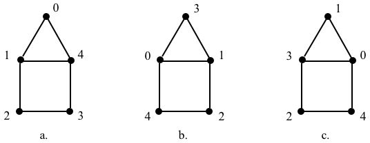
We can represent these instances of \(G\) using, for example, \(AVL\)s:

{0:[1,4], 1:[0,2,4], 2:[1,3], 3:[2,4], 4:[0,1,3]} # AVL_a
{0:[1,4], 1:[0,2], 2:[1,3,4], 3:[2,4], 4:[0,2,3]} # AVL_b
{0:[1,4], 1:[0,2,4], 2:[1,3], 3:[2,4], 4:[0,1,3]} # AVL_c

We can think of the permutation \(P_{i \rightarrow j}\) as a function \(\pi(x)\) that maps \(x\), the label of a vertex of \(G_i\), onto a unique label \(y\) of vertex of \(G_j\). For example, we can think of the permutation
$$
P_{a \rightarrow b}=
\left(
\begin{array}{c}
0,1,2,3,4\\
3,0,4,2,1
\end{array}
\right)
$$
that maps \(G_a\) onto \(G_a\) as the function \(\pi(x)\):
$$
\begin{array}{c}
\pi(0)=3\\
\pi(1)=0\\
\pi(2)=4\\
\pi(3)=2\\
\pi(4)=1\\
\end{array}
$$

Inversion

Permutations are functions that operate over the labels of the graph and map a set of labels onto a shuffling of those same labels. The following permutations \(P_{i\rightarrow j}\) in two-line notation map the labels of the vertices of \(G_i\) onto those of \(G_j\):

$$
P_{a \rightarrow b}=
\left(
\begin{array}{c}
0,1,2,3,4\\
3,0,4,2,1
\end{array}
\right)~~~~~~~~~
P_{b \rightarrow c}=
\left(
\begin{array}{c}
0,1,2,3,4\\
3,0,4,1,2
\end{array}
\right)~~~~~~~~~
P_{a \rightarrow c}=
\left(
\begin{array}{c}
0,1,2,3,4\\
1,3,2,4,0
\end{array}
\right)
$$

The inverse of a permutation reverses the direction of the permutation, e.g., given a permutation \(P_{i\rightarrow j}\), we want to find the permutation \(P_{j\rightarrow i}\), i.e., we are looking for the permutation that maps the labels of \(G_j\) back onto those of \(G_i\). In terms of our function \(\pi(x)\), we are looking for its inverse \(\pi^{-1}(x)\). For example,
$$
\begin{array}{c}
\pi(0)=3\\
\pi(1)=0\\
\pi(2)=4\\
\pi(3)=2\\
\pi(4)=1\\
\end{array}
~~~~\Longrightarrow~~~~~
\begin{array}{c}
\pi^{-1}(3)=0\\
\pi^{-1}(0)=1\\
\pi^{-1}(4)=2\\
\pi^{-1}(2)=3\\
\pi^{-1}(1)=4\\
\end{array}
~~~~=~~~~~
\begin{array}{c}
\pi^{-1}(0)=1\\
\pi^{-1}(1)=4\\
\pi^{-1}(2)=3\\
\pi^{-1}(3)=0\\
\pi^{-1}(4)=2\\
\end{array}
$$

In our case, since we have the diagrams of the labeled graphs at our disposal, we can find their inverses by inspection:

$$
P_{b \rightarrow a}=
\left(
\begin{array}{c}
0,1,2,3,4\\
1,4,3,0,2
\end{array}
\right)~~~~~~~~~
P_{c \rightarrow b}=
\left(
\begin{array}{c}
0,1,2,3,4\\
1,3,4,0,2
\end{array}
\right)~~~~~~~~~
P_{c \rightarrow a}=
\left(
\begin{array}{c}
0,1,2,3,4\\
4,0,2,1,3
\end{array}
\right)
$$

Now let’s assume that that we do not have the diagrams of the graphs but only the direct permutation, i.e., the permutation \(P_{i\rightarrow j}\), and we want its inverse, i.e., \(P_{j\rightarrow i}\). If we have the permutation in two-line notation, we swap the rows and, if we want to, we sort the columns:

$$
P_{b \rightarrow a}=
\left(
\begin{array}{c}
0,1,2,3,4\\
3,0,4,2,1
\end{array}
\right)~~~~\Longrightarrow~~~~~
P_{b \rightarrow a}=
\left(
\begin{array}{c}
3,0,4,2,1\\
0,1,2,3,4
\end{array}
\right)~~~~=~~~~
\left(
\begin{array}{c}
0,1,2,3,4\\
1,4,3,0,2
\end{array}
\right)
$$

If we have the permutation in one-line notation, we convert it into two-line notation, invert it, sort the columns, and remove the top row. For example, the following pairs are inverses of each other

[3,0,4,2,1] # P_a_b
[1,4,3,0,2] # p_b_a

[3,0,4,1,2] # P_b_c
[1,3,4,0,2] # p_c_b

[1,3,2,4,0] # P_a_c
[4,0,2,1,3] # p_c_a

To invert a permutation in cycle notation, we reverse the elements of each cycle; for example, to find the inverse of \(P_{b \rightarrow c}\) we reverse its cycles:
$$
P_{b \rightarrow c}=
(0,3,1)(2,4)
~~~~\Longrightarrow~~~~~
P_{c \rightarrow b}=
(1,3,0)(4,2)
$$
If we want to, we can rotate the elements of each cycle to have the smaller element first, e.g.,
$$
P_{c \rightarrow b}=
(1,3,0)(4,2) = (0,1,3)(2,4)
$$
Finaly, we can sort the cycles themselves, in ascending order, using the first element of each cycle as the sorting key. In our example, 0 < 2 so they cycles are already sorted.The pairs of inverses for our examples are:

[[0,3,2,4,1]]   # P_a_b
[[0,1,4,2,3]]   # p_b_a

[[0,3,1],[2,4]] # P_b_c
[[0,1,3],[2,4]] # p_c_b

[[0,1,3,4]]     # P_a_c
[[0,4,3,1]]     # p_c_a

Finally, if we are using permutation matrices then we transpose the matrix because, for permutation matrices, inverses are the same as transposes. For example,
$$
P_{a \rightarrow b}=
\left|
\begin{array}{ccccc}
0&1&0&0&0\\
0&0&0&0&1\\
0&0&0&1&0\\
1&0&0&0&0\\
0&0&1&0&0\\
\end{array}
\right|
~~~~\Longrightarrow~~~~~
P_{b \rightarrow a}=P_{a \rightarrow b}^{-1}=P_{a \rightarrow b}^T=
\left|
\begin{array}{ccccc}
0&0&0&1&0\\
1&0&0&0&0\\
0&0&0&0&1\\
0&0&1&0&0\\
0&1&0&0&0\\
\end{array}
\right|
$$

We will not delve into the rabbit hole of which way to invert a permutation is more efficient because it depends on what we are working with. By itself, the most efficient inversion procedure is to invert the cycle representation that in the best case has no cost and in the worst is linear, while the least efficient is the matrix transpose that has a fixed cost of \(O(n^2)\), unless we are using some sparse matrix representation, which has its own associated overhead.

Composition

A permutation composition, a.k.a., permutation product, is the process of permuting a permutation, i.e., of chaining permutations. For example, we can describe the permutations \(P_{a \rightarrow b}\), \(P_{b \rightarrow c}\) and \(P_{a \rightarrow c}\) given by

$$
P_{a \rightarrow b}=
\left(
\begin{array}{c}
0,1,2,3,4\\
3,0,4,2,1
\end{array}
\right)~~~~~~~~~
P_{b \rightarrow c}=
\left(
\begin{array}{c}
0,1,2,3,4\\
3,0,4,1,2
\end{array}
\right)~~~~~~~~~
P_{a \rightarrow c}=
\left(
\begin{array}{c}
0,1,2,3,4\\
1,3,2,4,0
\end{array}
\right)
$$

with the functions \(\pi(x)\), \(\sigma(x)\) and \(\tau(x)\), respectively:

$$
\begin{array}{c}
\pi(0)=3\\
\pi(1)=0\\
\pi(2)=4\\
\pi(3)=2\\
\pi(4)=1\\
\end{array}
~~~~~~~~~
\begin{array}{c}
\sigma(0)=3\\
\sigma(1)=0\\
\sigma(2)=4\\
\sigma(3)=1\\
\sigma(4)=2\\
\end{array}
~~~~~~~~~
\begin{array}{c}
\tau(0)=1\\
\tau(1)=3\\
\tau(2)=2\\
\tau(3)=4\\
\tau(4)=0\\
\end{array}
$$

Now, since \(P_{a \rightarrow b}\) maps the labels of \(G_a\) to those of \(G_b\), and \(P_{b \rightarrow c}\) maps the labels of \(G_b\) to those of \(G_c\), it stands to reason that their composition \(P_{a \rightarrow c}\), i.e., chaining them, will map the labels of \(G_a\) to those of \(G_c\), i.e.,
$$
P_{a \rightarrow b}~\circ~P_{b \rightarrow c} = P_{a \rightarrow c}
$$
where \(\circ\) denotes the composition operation, or, using functions:
$$
\sigma(\pi(x)) = \tau(x)
$$

Hence, to find \(P_{a \rightarrow c}\) we permute \(P_{a \rightarrow b}\) by \(P_{b \rightarrow c}\):

$$
\begin{array}{c}
\tau(0)=\sigma(\pi(0))=\sigma(3)=1\\
\tau(1)=\sigma(\pi(1))=\sigma(0)=3\\
\tau(2)=\sigma(\pi(2))=\sigma(4)=2\\
\tau(3)=\sigma(\pi(3))=\sigma(2)=4\\
\tau(4)=\sigma(\pi(4))=\sigma(1)=0\\
\end{array}
$$
that, indeed, is \(P_{a \rightarrow c}\).

With two-line notation, we rearrange the columns of \(P_{b \rightarrow c}\) such that its first row matches the last row of \(P_{a \rightarrow b}\), and then form \(P_{a \rightarrow c}\) as the first row of \(P_{a \rightarrow b}\) and the last row of \(P_{b \rightarrow c}\):
$$
\left.
\begin{array}{c}
P_{a \rightarrow b}
~=~
\left(
\begin{array}{c}
0,1,2,3,4\\
3,0,4,2,1
\end{array}
\right)
~=~
\left(
\begin{array}{c}
0,1,2,3,4\\
3,0,4,2,1
\end{array}
\right)
\\
\\
P_{b \rightarrow c}
~=~
\left(
\begin{array}{c}
0,1,2,3,4\\
3,0,4,1,2
\end{array}
\right)
~=~
\left(
\begin{array}{c}
3,0,4,1,2\\
1,3,2,0,4
\end{array}
\right)
\end{array}
\right\}
~~
\left(
\begin{array}{c}
0,1,2,3,4\\
1,3,2,4,0
\end{array}
\right)
~=~
P_{a \rightarrow c}
$$

Composition of permutation matrices is as follows. We saw that
$$
P_{a \rightarrow b}~\mbox{AVM}_a~P_{a \rightarrow b}^T = \mbox{AVM}_b
$$
Likewise,
$$
P_{b \rightarrow c}~\mbox{AVM}_b~P_{b \rightarrow c}^T = \mbox{AVM}_c
$$
Hence, replacing the former on the later:
$$
P_{b \rightarrow c}~(P_{a \rightarrow b}~\mbox{AVM}_a~P_{a \rightarrow b}^T)~P_{b \rightarrow c}^T = \mbox{AVM}_c
$$
which we can rewrite as
$$
(P_{b \rightarrow c}~P_{a \rightarrow b})~\mbox{AVM}_a~(P_{a \rightarrow b}^T~P_{b \rightarrow c}^T) = \mbox{AVM}_c
$$
Since \(A^TB^T=(BA)^T\) for any matrices \(A\) and \(B\), then
$$
(P_{b \rightarrow c}~P_{a \rightarrow b})~\mbox{AVM}_a~(P_{b \rightarrow c}~P_{a \rightarrow b})^T = \mbox{AVM}_c
$$
or
$$
P_{a \rightarrow c}~\mbox{AVM}_a~P_{a \rightarrow c}^T = \mbox{AVM}_c
$$
with
$$
P_{a \rightarrow c} = P_{b \rightarrow c}~P_{a \rightarrow b}
$$
Explicitly:
$$
P_{b \rightarrow c}~P_{a \rightarrow b}=
\left|
\begin{array}{ccccc}
0&1&0&0&0\\
0&0&0&1&0\\
0&0&0&0&1\\
1&0&0&0&0\\
0&0&1&0&0\\
\end{array}
\right|
\left|
\begin{array}{ccccc}
0&1&0&0&0\\
0&0&0&0&1\\
0&0&0&1&0\\
1&0&0&0&0\\
0&0&1&0&0\\
\end{array}
\right|
=
\left|
\begin{array}{ccccc}
0&0&0&0&1\\
1&0&0&0&0\\
0&0&1&0&0\\
0&1&0&0&0\\
0&0&0&1&0\\
\end{array}
\right|
=P_{a \rightarrow c}
$$

In Python, using straight (and expensive) matrix multiplication:

import numpy as np
P_b_c = np.array([[0,1,0,0,0],[0,0,0,1,0],[0,0,0,0,1],[1,0,0,0,0],[0,0,1,0,0]])
P_a_b = np.array([[0,1,0,0,0],[0,0,0,0,1],[0,0,0,1,0],[1,0,0,0,0],[0,0,1,0,0]])
P_a_c = P_b_c @ P_a_b
print(P_a_c)

Again, in practice, everytime we write down a multiplication of a matrix M by a permutation matrix, we avoid doing the actual multiplication and instead simply permute the rows or columns of M.

First published on Feb. 18/2026