The many ways to label a graph
Would you like to know more?
The word permutation has two meanings in math. The first one is a shuffling of a sequence of elements, in our case, the shuffling of the labels of the vertices. It is totally up to us how to label an unlabeled graph because, under the hood, all possible labelings represent the same unlabeled graph. Consider three different labelings \(G_a\), \(G_b\), and \(G_c\) of the same unlabeled graph \(G\):
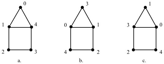
If the order of graph \(G\) is \(n\), then we can shuffle the labels of its vertices in \(n!\) possible different ways, i.e., there are \(n!\) permutations. In our example, since the order of \(G\) is \(n=5\), there are \(n! = 120\) possible permutations and thus, 120 different labelings; indeed, we can first label any one vertex with any of the 5 labels, and then label another vertex with any of 4 remaining labels, then a third one with any of the 3 remaining labels, and so on; the labelings of \(G\) shown as \(G_a\), \(G_b\), and \(G_c\), are 3 of these 120 possible labelings. Their AVLs are:
{0:[1,4], 1:[0,2,4], 2:[1,3], 3:[2,4], 4:[0,1,3]} # AVL_a
{0:[1,3,4], 1:[0,2,3], 2:[1,4], 3:[0,1], 4:[0,2]} # AVL_b
{0:[1,3,4], 1:[0,3], 2:[3,4], 3:[0,1,2], 4:[0,2]} # AVL_c
Cauchy’s two-line notation
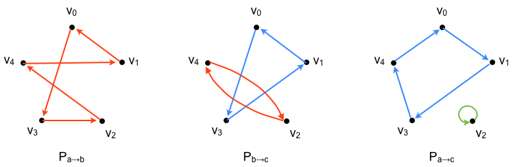
We can describe permutations using Cauchy’s two-line notation: the top row contains the elements of the permutation, i.e., our labels, while the bottom row contains their mappings; for example, the permutations \(P_{i\rightarrow j}\) that transform the labels of \(G_i\) into the labels of \(G_j\) are:
$$
P_{a \rightarrow b}=
\left(
\begin{array}{c}
0,1,2,3,4\\
3,0,4,2,1
\end{array}
\right)~~~~~~~~~
P_{b \rightarrow c}=
\left(
\begin{array}{c}
0,1,2,3,4\\
3,0,4,1,2
\end{array}
\right)~~~~~~~~~
P_{a \rightarrow c}=
\left(
\begin{array}{c}
0,1,2,3,4\\
1,3,2,4,0
\end{array}
\right)
$$
The following graphs show the transitions of these vertices as arcs. For example, for \(P_{a \rightarrow b}\) we have that \(v_0\) of \(G_a\) becomes \(v_3\) of \(G_b\), \(v_1\) of \(G_a\) becomes \(v_0\) of \(G_b\), and so on, while for \(P_{b \rightarrow c}\) we have that \(v_0\) of \(G_b\) becomes \(v_3\) of \(G_c\), and so on.
Since the pairing between the elements of the top and bottom rows is explicit, we can shuffle the columns of a given permutation into other equally valid representations, e.g.,
$$
P_{a \rightarrow b}=
\left(
\begin{array}{c}
0,1,2,3,4\\
3,0,4,2,1
\end{array}
\right) =
\left(
\begin{array}{c}
1,2,4,3,0\\
0,4,1,2,3
\end{array}
\right)=
\left(
\begin{array}{c}
3,1,0,2,4\\
2,0,3,4,1
\end{array}
\right)
$$
Usually there is no reason to do this shuffling, though, so our default is to use the representation whose top row in sorted in ascending order.
The identity permutation, a.k.a. the trivial permutation, maps the labels of the original AVL onto themselves so we have
$$
I =
\left(
\begin{array}{c}
0,1,2,3,4\\
0,1,2,3,4
\end{array}
\right)
$$
One-line notation
Let’s assume that we are representing permutations using the Cauchy’s two-line notation in which the top rows are sorted; in such a case, we already know what the row top is and we can omit writing it and, instead, simply describe the permutation using the bottom row:
$$
P_{a \rightarrow b}=
3,0,4,2,1
~~~~~~~~~
P_{b \rightarrow c}=
3,0,4,1,2
~~~~~~~~~
P_{a \rightarrow c}=
1,3,2,4,0
$$
or, as Python one-liners:
[3,0,4,2,1] # p(a->b)
[3,0,4,1,2] # p(b->c)
[1,3,2,4,0] # p(a->c)
The identity permutation is
$$
I =
0,1,2,3,4
$$
or, as a Python one-liner:
[0,1,2,3,4] # Identity permutation
Cycle notation
Looking back at the diagrams of transitions of our sample permutations, we can see that the transition of vertices of \(P_{a \rightarrow b}\) forms a sequence of the five vertices that repeats itself, i.e., \(v_0\) becomes \(v_3\), which becomes \(v_2\), which becomes \(v_4\), which becomes \(v_1\), which becomes \(v_0\), and then the sequence repeats. These closed transitions are called cycles or orbits. A cycle with \(k\) elements is called a k-cycle. A degeneracy is a cycle that contains all the elements of the permutation so, for example, the permutation \(P_{a \rightarrow b}\) has a single cycle – a 5-cycle – that is a degeneracy.
Cycles can involve any number of vertices, but the cycles of a permutation are such that the vertices in one cycle do not appear in any other cycle, and that every vertex belongs to a cycle. For example, for \(P_{b \rightarrow c}\), there is a 3-cycle in which \(v_3\) becomes \(v_1\), which becomes \(v_0\), which cycles back to become \(v_3\); and a 2-cycle, where \(v_2\) becomes \(v_4\), which cycles back to become \(v_2\). An exchange of exactly two vertices like this last one, i.e., a 2-cycle, is called a transposition, so the permutation \(P_{b \rightarrow c}\) has a 3-cycle and a transposition.
Finally, we have the 1-cycles, a.k.a. fixed points. For \(P_{a \rightarrow c}\), there is 4-cycle that covers \(v_0\), \(v_1\), \(v_3\) and \(v_4\); \(v_2\) is a vertex that doesn’t change places during the permutation so it’s cycle is \((2)\); we actually don’t write fixed points in the cycle notation because we simply assume that every absent element is a fixed point; this is what makes the cycle notation compact. Hence, we could write \(P_{a \rightarrow c}\) as \((0,4,3,1)(2)\) but normally we will omit the fixed point and simply write it as \((0,4,3,1)\)
Hence, the cycle notation is a succint way to write permutations in which we write down their cycles but omit their fixed points; for our examples we have:
$$
P_{a \rightarrow b}=
\begin{array}{c}
(0,3,2,4,1)
\end{array}
~~~~~~~~~
P_{b \rightarrow c}=
\begin{array}{c}
(0,3,1)(2,4)
\end{array}
~~~~~~~~~
P_{a \rightarrow c}=
\begin{array}{c}
(0,1,3,4)
\end{array}
$$
or, in Python:
[[0,3,2,4,1]]    # p(a->b)
[[0,3,1],[2,4]]  # p(b->c)
[[0,1,3,4]]      # p(a->c)
Every vertex under the identity permutation is a fixed point, which we don’t write in cycle notation, so the identity permutation in cycle notation is simply the empty list:
[ ] # identity permutation
Our use of Python lists to represent permutations in both one-line and cycle notations should not cause any confusion, i.e., permutations in one-line notations are lists while permutation in cycle notation are lists of lists.
Permutation Matrices
Consider the AMV of the graph \(G_a\); in the page of Representation of graphs we obtained its \(\mbox{AVM}\); we can also write the \(\mbox{AVM}\) of \(G_b\) that we find at the beginning of these page. These two matrices are:
$$\mbox{AVM}_a =
\left|
\begin{array}{ccccc}
0&1&0&0&1\\
1&0&1&0&1\\
0&1&0&1&0\\
0&0&1&0&1\\
1&1&0&1&0\\
\end{array}
\right|
~~~~~~~~
\mbox{AVM}_b =
\left|
\begin{array}{ccccc}
0&1&0&1&1\\
1&0&1&1&0\\
0&1&0&0&1\\
1&1&0&0&0\\
1&0&1&0&0\\
\end{array}
\right|
$$
The permutation \(P_{a \rightarrow b}\) tells us how the labels of \(G_a\) map onto those of \(G_b\):
$$
P_{a \rightarrow b}=
\left(
\begin{array}{c}
0,1,2,3,4\\
1,4,3,0,2
\end{array}
\right)
$$
We can represent this permutation using a matrix in a couple of ways; first, we start with a zero matrix of order \(n\) and, using the Cauchy’s two-line notation, we set to 1 the entry of the row indicated by the top row label and the column indicated by the bottom row label, e.g., we place ones at (0,1), (1,4), (2,3), (3,0) and (4,2); let’s call this permutation matrix \(P_{a \rightarrow b}\). Alternatively, we can use the columns instead of the rows, e.g., we place ones at (1,0), (4,1), (3,2), (0,3) and (2,4); let’s call it \(Q_{a \rightarrow b}\):
$$P_{a \rightarrow b} =
\left|
\begin{array}{ccccc}
0&1&0&0&0\\
0&0&0&0&1\\
0&0&0&1&0\\
1&0&0&0&0\\
0&0&1&0&0\\
\end{array}
\right|
~~~~~~~
Q_{a \rightarrow b} =
\left|
\begin{array}{ccccc}
0&0&0&1&0\\
1&0&0&0&0\\
0&0&0&0&1\\
0&0&1&0&0\\
0&1&0&0&0\\
\end{array}
\right|
$$
Permutation matrices, like \(P_{a \rightarrow b}\) and \(Q_{a \rightarrow b}\), have certain characteristics. For example, a permutation matrix is binary, it has exactly one 1 per row and column, and its inverse is equal to its transpose. In our case, \(P_{a \rightarrow b}\) and \(Q_{a \rightarrow b}\) happen to be the transpose, and thus the inverse, of each other.
As you might have guessed, the identity permutation matrix is simply the identity matrix:
$$P_I=
\left|
\begin{array}{ccccc}
1&0&0&0&0\\
0&1&0&0&0\\
0&0&1&0&0\\
0&0&0&1&0\\
0&0&0&0&1\\
\end{array}
\right|
$$
Permuting AVLs
Above we saw examples of the first meaning of permutation, i.e., a sequence that has been shuffled from an original order. The second meaning of permutation is the actual process of shuffling the elements from one sequence to another one. At the top of this page there is a program that permutes AVLs. For example, paste \(\mbox{AVL}_a\),
{0:[1,4], 1:[0,2,4], 2:[1,3], 3:[2,4], 4:[0,1,3]} # AVL_a
select the custom radio button, and paste the \(P_{a \rightarrow b}\) permutation in a one-line notation,
[3,0,4,2,1] # p(a->b)
When we run the program, we get back \(\mbox{AVL}_b\):
{0:[1,3,4], 1:[0,2,3], 2:[1,4], 3:[0,1], 4:[0,2]} # AVL_b
Now, this is how it is done. We have two different representations of a graph: the \(AVL\) and the \(AVM\). To permute the labels using the \(AVL\), we replace its labels with their corresponding permuted labels, as described by the two-line permutation, e.g., to permute \(\mbox{AVL}_a\) into \(\mbox{AVL}_b\) we replace the labels of \(\mbox{AVL}_a\) according to the permutation
$$
P_{a \rightarrow b}=
\left(
\begin{array}{c}
0,1,2,3,4\\
3,0,4,2,1
\end{array}
\right)
$$
to obtain
{3:[0,1], 0:[3,4,1], 4:[0,2], 2:[4,1], 1:[3,0,2]} # AVL_b
This is already the correct result, i.e., \(\mbox{AVL}_b\). Still, to get the nice sorted version that we use, we sort the tuples:
{3:[0,1], 0:[1,3,4], 4:[0,2], 2:[1,4], 1:[0,2,3]} # AVL_b
and sort the keys:
{0:[1,3,4], 1:[0,2,3], 2:[1,4], 3:[0,1], 4:[0,2]} # AVL_b
Permuting AVMs
If we are working with the \(AVM\) instead of the \(AVL\), we need to exchange the rows and columns of one \(\mbox{AVM}\) into those of the other \(\mbox{AVM}\). Premultiplying a matrix \(A\) by a permutation matrix exchanges the rows of \(A\), while postmultiplying \(A\) by a permutation matrix exchanges the columns of \(A\). In our example, we need to premultiply \(\mbox{AVM}_a\) by the permutation matrix \(P_{a \rightarrow b}\) and postmultiply it by \(Q_{a \rightarrow b}\), which happens to be the transpose of \(P_{a \rightarrow b}\). Hence we have:
$$
P_{a \rightarrow b}~\mbox{AVM}_a~Q_{a \rightarrow b} = P_{a \rightarrow b}~\mbox{AVM}_a~P_{a \rightarrow b}^T = \mbox{AVM}_b
$$
or, explicitly,
$$
\left|
\begin{array}{ccccc}
0&1&0&0&0\\
0&0&0&0&1\\
0&0&0&1&0\\
1&0&0&0&0\\
0&0&1&0&0\\
\end{array}
\right|
~
\left|
\begin{array}{ccccc}
0&1&0&0&1\\
1&0&1&0&1\\
0&1&0&1&0\\
0&0&1&0&1\\
1&1&0&1&0\\
\end{array}
\right|
~
\left|
\begin{array}{ccccc}
0&1&0&0&0\\
0&0&0&0&1\\
0&0&0&1&0\\
1&0&0&0&0\\
0&0&1&0&0\\
\end{array}
\right|^T
=
\left|
\begin{array}{ccccc}
0&1&0&1&1\\
1&0&1&1&0\\
0&1&0&0&1\\
1&1&0&0&0\\
1&0&1&0&0\\
\end{array}
\right|
$$
In Python, using straight (and expensive) matrix multiplication:
import numpy as np
P = np.array([[0,1,0,0,0],[0,0,0,0,1],[0,0,0,1,0],[1,0,0,0,0],[0,0,1,0,0]])
AVM_a = np.array([[0,1,0,0,1],[1,0,1,0,1],[0,1,0,1,0],[0,0,1,0,1],[1,1,0,1,0]])
AVM_b = P @ AVM_a @ P.T
print(AVM_b)
Matrix multiplication is straightfoward but expensive; in Python, we can do better permuting the \(\mbox{AVM}\) using the one-line permutation array and the slicing function of numpy:
import numpy as np
P = np.array([1,4,3,0,2])
AVM_a = np.array([[0,1,0,0,1],[1,0,1,0,1],[0,1,0,1,0],[0,0,1,0,1],[1,1,0,1,0]])
AVM_b = AVM_a[P,:][:,P]
print(AVM_b)
In practice, everytime we write down a multiplication of a matrix \(M\) by a permutation matrix, we avoid doing the actual multiplication and instead simply permute the rows or columns of \(M\).
First published on Feb. 5/2026