Bringing graphs to the digital age
Would you like to know more?
We can represent relationships among elements using graphs, e.g., traveling routes among cities, chemical bonds between atoms, links between websites, relationships with friends and family, etc. So far we have seen the analog graphical representations of graphs, i.e., drawings of dots, which represent elements, connected by arrows or edges, which represent one- or two-way relationships. To study graphs using a computer we need to represent vertices, arcs and edges digitally, as numbers.
The graphs that we have seen so far do not have labeled vertices or edges, i.e., they are unlabeled graphs. To study and storage graphs we can label their vertices, thus obtaining a labeled graph. The order \(n\) of a graph is the number of vertices that it has; we will label these \(n\) vertices as \({0, 1, …, n-1}\), and refer to them as \(v_0\), \(v_1\), …, \(v_{n-1}\) [*]. Another possibility is to label the edges, but such representation is less common than labeling the vertices.
Once we have labeled the vertices of a graph, we can represent it using an adjacency vertex list, or AVL. We say that a vertex \(v_i\) is adjacent to a vertex \(v_j\) if there is an arc from \(v_i\) to \(v_j\); the fact that \(v_i\) is adjacent to \(v_j\) doesn’t mean that \(v_j\) is adjacent to \(v_i\). If \(v_i\) and \(v_j\) are connected by an edge, then the connection is symmetric because an edge is simply two arcs traveling in opposite directions between those two vertices, i.e., there is an arc from \(v_i\) to \(v_j\) and another from \(v_j\) to \(v_i\); we count separately each arc between any two vertices.
The adjacency vertex list (AVL) is usually simply called the adjacency list, but we specify it here because there is also a less-often-used adjacency edge list. If there are several versions of a graph \(G\), e.g., \(G_a\), \(G_b\), etc., we will denote their AVLs as \(\mbox{AVL}_{G_a}\), \(\mbox{AVL}_{G_b}\), etc., or, if there is no risk of confusion, \(\mbox{AVL}_a\), \(\mbox{AVL}_b\), etc.
Let’s represent an unlabeled simple undirected graph with an AVL. First we label the vertices in an arbitrary way, e.g., we’ll label them counterclockwise starting from the top. Then we map the edges as arcs so we can tell the adjacency between vertices.
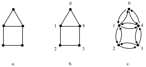
Let’s call the graph above \(G\), our default name for a graph; it’s AVL is
$$
\begin{array}{ll}
0:&1,4\\
1:&0,2,4\\
2:&1,3\\
3:&2,4\\
4:&0,1,3\\
\end{array}
$$
or, as a one-line Python hash table:
{0:[1,4], 1:[0,2,4], 2:[1,3], 3:[2,4], 4:[0,1,3]} # G
We could have represented the AVL using a list, but the hash table representation tell us at a glance the adjacent vertices of a particular vertex, e.g., there is an arc from \(v_2\) to each of \(v_1\) and \(v_3\). The # character at the end of the one-liner AVL and the text that follows it are a Python comment; we can ignore it or omit it.
A second way to represent a graph is using the adjacency vertex matrix, or AVM. This is an \(n \times n\) matrix in which each of the \(n\) rows corresponds to a vertex from which an arc departs and each of the \(n\) columns corresponds to the vertex to which the arc arrives, i.e., the entry \((i,j)\) in the matrix is the number of arcs that depart \(v_i\) and arrive to \(v_j\). For example, the AVM of \(G\), or \(\mbox{AVM}_G\), is
$$\mbox{AVM}_G =
\left|
\begin{array}{ccccc}
0&1&0&0&1\\
1&0&1&0&1\\
0&1&0&1&0\\
\textbf{0}&\textbf{0}&\textbf{1}&\textbf{0}&\textbf{1}\\
1&1&0&1&0\\
\end{array}
\right|
$$
We can see the one-to-one correspondence between \(\mbox{AVL}_G\) and \(\mbox{AVM}_G\), e.g., \(\mbox{AVL}_G\) says is that there are single arcs departing \(v_3\) and arriving to each of \(v_2\) and \(v_4\), while the entries \((3,2)\) and \((3,4)\) of \(\mbox{AVM}_G\) have a 1, indicating this same fact; the rest of the entries in the third row are 0 indicating that there are no arcs departing \(v_3\) and arriving to any vertex other than \(v_2\) and \(v_4\).
AVMs of undirected graphs are always symmetric because if there is an arc from \(v_i\) to \(v_j\) then there is a corresponding returning arc from \(v_j\) to \(v_i\), while AVMs of digraphs are not symmetric. Also, AVMs of simple graphs are binary while those of multigraphs are not.
AVMs play a crucial role in the study of graphs because we can answer certain queries easily with them. For example, consider the following scene from “Good Will Hunting”, where a math professor is asking questions about the graph \(G\), a 4-vertex undirected multigraph, shown on the top-left of the board; it has double edge between vertices 2 and 3; its vertices are labeled from 1 to 4. The questions and answers are on the left and right sides, respectively:
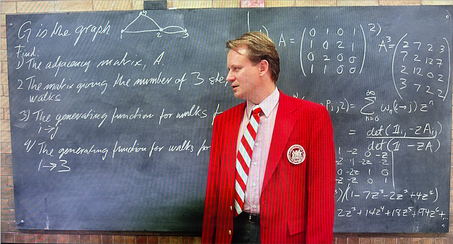
Let’s focus on questions 1 and 2. The first question asks for the adjacency matrix of \(G\), i.e., the \(\mbox{AVM}_G\), and the answer is
$$\mbox{AVM}_G =
\left|
\begin{array}{cccc}
0&1&0&1\\
1&0&2&1\\
0&2&0&0\\
1&1&0&0\\
\end{array}
\right|$$
No mistery here: the matrix is symmetric because \(G\) is undirected, and is not binary because \(G\) is not simple; the 2s in the (2,3) and (3,2) entries denote the double edge between \(v_2\) and \(v_3\).
The second question asks what is the matrix giving the number of 3-step walks. A 3-step walk between \(v_i\) and \(v_j\) is a way in which we can depart from \(v_i\), walk 3 steps, and end up at \(v_j\). For example, there are 2 ways we can depart from \(v_1\), take 3 steps, and end up at \(v_1\) again, namely (1,4,2,1) and (1,2,4,1); likewise, there are 3 ways in which we can depart from \(v_1\), take 3 steps, and end up at \(v_4\), namely (1,4,1,4), (1,4,2,4) and (1,2,1,4). Finding this information using AVLs is difficult compared with computing the cube of the adjacency vertex matrix \(A\), which provides the correct answer, e.g., \(A^3[1,1]=2\) and \(A^3[1,4]=3\). AVMs occupy a lot of space, though, so we will stick with AVLs as much as possible. Let’s now retake the use of \(G\) as the name of our example, instead of the one from the movie.
Now that we can identify individual vertices, we can characterize them. The most basic feature of a vertex is its degree, a.k.a. its valency. If we are dealing with a digraph, the out-degree is the number of arcs that leave the vertex, while the in-degree is the number of arcs that arrive to it; if we are dealing with an undirected graph, the out-degree is the same as the in-degree, so we just call it the degree of the vertex, and we can define it simply as the number of edges connected to the vertex. For example, for our graph \(G\), the degree of \(v_0\) is 2, while the degree of \(v_1\) is 3.
A more general example is that of an unlabeled disconnected pseudo digraph with multiple loops, edges and isolated vertices. Again, we label the vertices in an arbitrary fashion, and then we recast the edges as arcs to find the vertex adjacency and arc multiplicity. For visualization purposes, we have colored the multiplicity tick marks in red. Again, let’s call it graph \(G\).
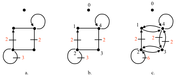
The AVL of the pseudograph \(G\) above is
{0:[], 1:[4], 2:[1,1,2,2,2,2,2,2,3], 3:[2,4,4], 4:[1,3,3,4]} # G
Vertex 0 has no adjacent vertices so its list is empty. For \(v_1\), there is one arc to \(v_4\). For \(v_2\), there are two arcs to \(v_1\), six arc loops from the three edge loops, and an arc to \(v_3\). For \(v_3\), there is an arc to \(v_2\) and two arcs to \(v_4\). And, finally, for \(v_4\) there is an arc to \(v_1\), two arcs to \(v_3\), and an arc loop.
Even though the subjects of graph theory are the abstract mathematical unlabeled graphs composed of a set of vertices and a set of connections between those vertices, we label them to study them. From here on, unless we specify otherwise, we will use the word “graph” to refer to graphs with labeled vertices, i.e., to labeled graphs.
Examples
The following are the AVLs of the graphs we saw in the definition page. We label the vertices counterclockwise, starting from the top, but this is arbitrary; all labelings are equivalent and represent the unlabeled graph equally well.
Simple connected graphs

{0:[1,4], 1:[0,2,4], 2:[1,3], 3:[2,4], 4:[0,1,3]} # a
{0:[1,4], 1:[], 2:[1,3], 3:[], 4:[1,3]}           # b
{0:[1,4], 1:[2,4], 2:[1,3], 3:[4], 4:[1,3]}       # c
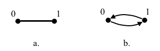
{0:[1], 1:[0]} # a
{0:[1], 1:[0]} # b
As expected, these two AVLs are identical since they are simply two different graphical representations of the same graph.
Simple disconnected graphs
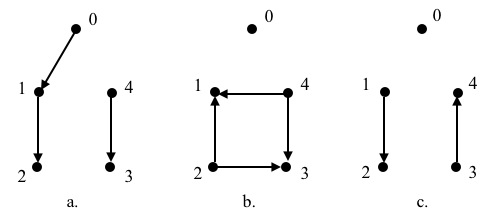
{0:[1], 1:[2], 2:[], 3:[], 4:[3]}      # a
{0:[], 1:[], 2:[1,3], 3:[], 4:[1,3]}   # b
{0:[], 1:[2], 2:[], 3:[4], 4:[]}       # c
Multigraphs
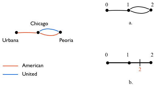
{0:[1], 1:[0,2,2], 2:[1,1]} # a
{0:[1], 1:[0,2,2], 2:[1,1]} # b
Multidigraphs
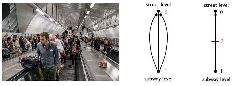
{0:[], 1:[0,0,0]} # a
{0:[], 1:[0,0,0]} # b
Loops
This is the simplest graph with a loop:
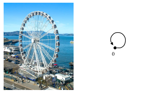
{0:[0]}
Pseudographs

{0:[], 1:[4], 2:[1,3], 3:[2,4], 4:[1,3,4]}                  # a
{0:[], 1:[4], 2:[1,1,3], 3:[4], 4:[1,3]}                    # b
{0:[], 1:[4], 2:[1,1,2,2,2,2,2,2,3], 3:[2,4,4], 4:[1,3,4]}  # c
[*] A note on label numbering
We label the vertices of a graph of order \(n\) as \(0, 1, \dots,n-1\), instead of the other option \(1,2,\dots,n\). I believe this difference originates from the differences between the Fortran and C computer languages. Fortran, an acronym of FORmula TRANslation, was designed to do math, while C was designed to write operating systems. Fortran indexes the arrays from 1 to n, designating the order of the entry, e.g., the first entry is 1, the second is 2, and so on, while C indexes the arrays with the distance to the beginning of the location of the array in memory, e.g., the first entry is 0 because there is a distance of 0 from the first element to the beginning of the array, the second entry is 1 because there is a distance of 1 from the second element to the beginning of the array, and so on. Both languages and its descendents, who inherited their indexing scheme, are popular. Which one is right? both and neither… it is simply a preference that mostly depends on the computer language that we normaly use. If we are working with Fortran or one of its descendents, then indexing arrays, matrices, and everything else starting at 1 feels natural, and if we are working with C or one of its descendents, then indexing arrays, matrices, and everything else starting at 0 feels equally natural. I usually program in C or Python, which is a descendent of C, so in my writing I use 0-based arrays and matrices. Aside from this, the first integer is 0, not 1.
First published on Dec. 19/2025