High-Symmetry graph maker

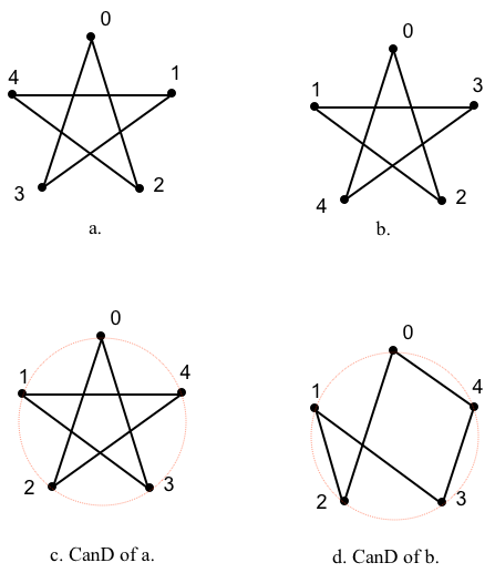
The mathematical concept of symmetry is that of a feature of an object that remains unchanged under a transformation like rotation or reflection, e.g., the letter W reflected about its vertical axis, or the letter S rotated 180° about its center. Graphs also exhibit symmetry, although it is not always apparent because a particular diagram of a graph might not display it. For example, consider the diagrams below.

The first diagram of this pentagram graph is symmetric when we rotate it about its center by any multiple of 72° and/or we flip it about, say, its vertical axis; on the other hand, the last three diagrams have a single symmetry, namely a flip about the vertical axis. However, all four of these are diagrams are from the same labeled pentagram graph, i.e., \(v_0\) is adjacent to \(v_2\) and \(v_3\), \(v_1\) is adjacent to \(v_3\) and \(v_4\), and so on.

We standarize the diagrams of a graph using a Canonical Drawing, a.k.a. a CanD, i.e., a drawing or layout of a labeled graph with the labels ordered in a circular fashion, at equal angles between them. All layouts of the same labeled graph have the same CanD, but it is perfectly possible, depending on the symmetries of the graph, for different labelings of the same graph to have different CanDs. For example, below, on the top row, we have two different labelings of the same pentagram graph, while on the bottom row we have their CanDs, which are not equal.

Many graphs lie in this category, with their various labelings having more that one CanD. This simply means that these graphs have an intermediate level of symmetry among their vertices and edges. We now look at the two extremes, i.e., symmetric graphs, for which all of its different labelings have the same CanD, and rigid graphs, for which all of its different labelings have a different CanD.

Symmetric graphs

A symmetric graph is one that is both edge and vertex transitive, i.e., every edge and vertex is indistinguishable from another. In contrast, we saw that two different labelings of the pentagram graph can have two different CanDs indicating that the vertices and/or edges of the pentragram graph are not transitive. Hence, the pentagram graph might be highly symmetric but it is not symmetric.

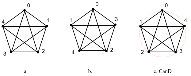
However, we can turn the labeled pentagram graphs of the example above into complete 5-vertex graphs, a.k.a., \(K_5\), without chaning their labels, by adding a pentagon to their perimeters. A complete graph is one in which every vertex is adjacent to every other vertex; complete graphs of order \(n\) are known as \(K_n\). The vertices and edges of our labeled graphs now are transitive and thus indistinguishable from each other, so they have the same CanD.

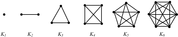
Here are the first six complete graphs, all of them symmetric; all the labeled diagrams of each of them will share the same CanD.

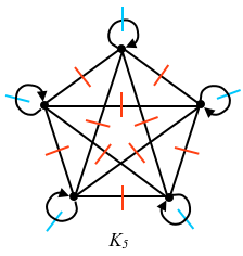
If we step aside from undirected graphs into directed pseudographs, we would have that every \(K_5\) graph of the form shown below is a complete graph, as long as all the red tick marks have the same multiplicity \(p\) and all the blue tick marks have the same multiplicity \(q\), for any non-negative \(p\) and \(q\). Hence, in general, we have that we can specify complete undirected pseudographs using the \(n\), \(p\) and \(q\) parameters, as \(K_n(p,q)\), e.g., the graph above would be \(K_5 = K_n(p,q)\) for \(n=5\), \(p=1\) and \(q=0\). Setting \(q\) to an even number would make this generalization of \(K_5\) an undirected graph.

Complete graphs are but one of many possible symmetric graphs, and we can carry a similar loop plus multiconnection analysis with each of such graphs.

In the context of undirected graphs, there are several families of highly symmetric graphs, each member of the family obtained by adjusting a couple of parameters. Some of the resulting graphs are symmetric, while others are only highly symmetric. Two such families are the Generalized Petersen graphs and the Johnson graphs; we can find a program at the top of this page to generate their AVLs.

The Generalized Petersen Graphs is a family of highly symmetric graphs based on two parameters \(n\) and \(k\); they are usually noted as \(G(n,k)\) or \(GPG(n,k)\). The following are some of these graphs, including the only seven graphs of this family that are symmetric:

These graphs have the following properties:

The Petersen G(24,5) is also in the Foster family of graphs, where it is known as the \(F_{048}A\); it is common for a given graph to be a member of various families of graphs.

The Johnson graphs are another family of highly symmetric graphs, also based on two parameters \(n\) and \(k\); they are usually noted as \(J(n,k)\). The following are some of these graphs:

The complexity of the Johnson graphs grows fast with \(n\) and \(k\). The order and size of a Johnson graph is
\[
\mbox{order}(J(n,k)) = {n \choose k}= \frac{n!}{k!(n-k)!},~~~~~~~~~\mbox{size}(J(n,k)) = \frac{1}{2}k(n-k){n \choose k}
\]

Hence, for the Johnson graphs above (and a few more) we have

The Johnson graphs includes the complete graphs because \(J(n,1) = K_n\), all of them symmetric; \(J(n,2)\) graphs are called n-triangular, while \(J(n,3)\) graphs are called n-tetrahedral Johnson graphs.

We can find a further list of symmetric graphs at Wolfram MathWorld.

Rigid graphs

On the opposite end of the spectrum of symmetric graphs, who have complete symmetry, we find the rigid graphs, a.k.a. asymmetric graphs or identity graphs, who have none. For a symmetric graph, any two vertices are indistinguishable from each other, and we can exchange them without changing the CanD, i.e., all n! labelings of a symmetric graph have the same CanD; in contrast, for a rigid graph any two vertices are unique in some way and we cannot transpose any two without altering the graph connectivity, i.e., each of the n! labelings of a rigid graph has its own unique CanD that is not shared with any other labeling. An example of an undirected rigid graph is the Frucht’s graph below:

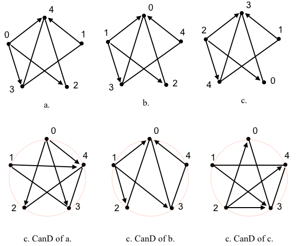
Now consider the digraph a. below; this digraph is rigid because the degree of \(v_n\) is \(n\), e.g., the degree of \(v_0\) is 0 because there are no arcs arriving to it, the degree of \(v_1\) is 1 because there is a single arc arriving to it, and so on. We take this digraph and, without changing the diagram, we relabel the vertices into the labeled digraphs in b. and c. Since the order of this digraph is 5, there are 5! = 120 different ways to label it, so a., b., and c. are only three of these 120 different labelings. And, each of the three has its own CanD; the other 117 labelings will also have their own unique CanDs.

We can build rigids graphs if we keep in mind that all we need is to make each vertex unique, so they cannot be transposed with any other vertex. A vertex can be unique in different ways. Above we set up a digraph whose vertices have different degrees. Below there are two ways to turn a symmetric general complete digraph into a rigid one.

In case a., all the vertices have a degree given by the \(p\) red tick marks, so we make each vertex unique by making all the \(q\) blue tick marks different; the result is a graph in which the order of every vertex differs from that of any other vertex by at least 1.

In case b. we use coloring, which is a technique to categorize vertices by coloring them in such a way that no two adjacent vertices have the same color. The minimum number of colors required to color a graph is called its chromatic number. For example, the chromatic number for a triangle, i.e., a.k.a. \(K_3\), is 3 because every vertex has to have a unique color; otherwise we would have at least two adjacent vertices with the same color. On the other hand, the chromatic number of a square is 2, because we can color each pair of opposite vertices with a different color and not have any adjacent vertex colored the same. Since every vertex of a complete graph of order \(n\) is adjacent to every other vertex, it follows that, as above, every complete graph has a chromatic number of \(n\), and since the color of every vertex of such colored complete graph is unique, then such graph is rigid.

A graph can be rigid in spite of having vertices with the same degrees, as the vertices might be unique due to their adjacencies. For example, consider the following graphs:

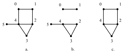
In a. \(v_5\) has a degree of 1, \(v_2\) has a degree of 3, and \(v_4\) has a degree of 4, which are not shared with any other vertex; on the other hand, \(v_0\), \(v_1\) and \(v_3\) have a degree of 2. The a. graph is rigid, though, because the vertices with shared degree are not transitive, i.e., in spite of their shared degree we can identify each one uniquely by its connections. Indeed, \(v_0\) is the only vertex of degree 2 adjacent to vertices of degrees 2 and 4, \(v_1\) is the only vertex of degree 2 adjacent to vertices of degrees 2 and 3, and \(v_3\) is the only vertex adjacent to degrees 3 and 4.

Graph b. is no longer rigid because \(v_0\) is indistinguishable from \(v_1\) and, \(v_2\) is indistinguishable from \(v_3\). Indeed, we can transpose \(v_0\) with \(v_1\), and \(v_2\) with \(v_3\) without changing the CanD.

Graph c. is no longer rigid either because, although \(v_0\) is disintguishable from \(v_1\), and \(v_2\) is distinguishable from \(v_4\), \(v_0\) and \(v_4\) together are indistinguishable from \(v_1\) and \(v_2\) together, i.e., the individual vertices are not transitive but the pairs are. This is displayed below, with a. showing the original graph. If we transpose the pair \(v_0\) and \(v_4\) with the pair \(v_1\) and \(v_2\), shown in b., we still have the same CanD, shown in c. However, if we transpose only \(v_0\) and \(v_1\), or only \(v_2\) and \(v_4\), shown in d. and e., we end up with a different CanD, shown in f.

In summary, we can use any characteristic that makes a vertex unique to determine if a graph is rigid; it might be its degree, its color, its connectivity, or anything else.

First published on Mar. 1/2026