Quick calculation of the ξ and Ω matrices for Graph-SLAM
The following is a quick way to derive the Ω and ξ matrices from the graph that describes the motion and measurement constraints or, alternatively, to use the graph to check if the matrices are correct.
Background
I took Udacity’s CS-373 class – Programming a Robotic Car – in March 2012. The class was taught by Sebastian Thrun, one of the most successful roboticists in many years, whose autonomous cars placed 1st and 2nd in the DARPA’s Grand Challenge and Urban Challenge, respectively.
The students of this course had access to a very active forum. I wrote a post about graph SLAM that many people liked so am reproducing here in case that new CS-373 Udacity students also find it useful.
SLAM stands for Simultaneous Localization and Mapping. It’s a technique that allows a robot to use repeated observations of landmarks to locate itself in a map of the environment built as it explores the surroundings.
In Graph-SLAM, the version of SLAM taught in CS-373, the robot motions and measurements are written as a set of linear equations
$$\xi = \Omega\cdot X$$
The matrices \(\Omega\) and \(\xi\) encode three type of constraints:
- Absolute Position
- Relative Position
- Relative Measurement of a landmark
The only known position of the robot is given by the Absolute Position constraint, commonly assigned to the initial position of the robot, i.e., \(x_0\), although I believe it could be assigned to any one position. Suppose that the robot moves to a new location by an amount \(d_{0\rightarrow1}\). Since \(x_0\) is an absolute reference, this would mean that the location of \(x_1\) is also known.
The problem is that there is an error associated with the motion and thus, we really do not know where the robot ended up at. Our best guess, though, is that the position \(x_1\) is at about
$$x_1 = x_0 + d_{0\rightarrow1}$$
We can build a chain of relative motions of this kind, each related to the next one by
$$x_{i+1} = x_i + d_{i\rightarrow {i+1}}$$
The observation of the landmarks from different locations \(x_i\) leads to similar constraints. A landmark \(L_j\) observed from position \(x_i\) at a distance \(k\) is described as
$$L_j = x_i + k$$
in which, again, we have that the relationship is only an approximation because of the uncertainty in both the location of the robot and the measurement.
Finally, depending on our confidence on a particular constraint we can add a weight to an equation, leading to a solution in which the error for that particular equation is reduced more than the others, e.g.,
$$W(L_j = x_i + k)$$
or
$$W L_j = Wx_i + Wk$$
We assign a large weigh to an equation (i.e., \(W > 1\)) when we believe that that particular equation has a small error (low variance) and should count more towards finding the solution of the system. Likewise, an equation associated with a large error (high variance) should be assigned a low weight (\( 0 < W < 1\)).
The \(\xi\) vector encodes the value of the constraint while the \(\Omega\) matrix encodes the locations that are involved in the constraint. Once the \(\xi\) and \(\Omega\) matrices are set up, we can solve for the vector \(X\) to obtain the absolute locations of the robot, i.e., the actual path that it followed, and the location of the landmarks, all with respect to the location set with the absolute position constraint.
The setup
In this example, taken straight from the course, the robot is moving along a line, on which the landmark \(L\) is also located. The robot is ordered to move certain distances along the line, and to measure its distance to the landmark \(L\):
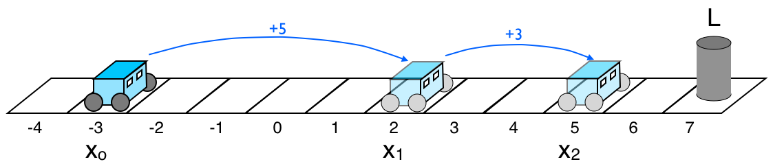
Initial position, and expected positions after motion commands
In an ideal world, the robot would move the desired distances accurately, and its measurements to the landmark \(L\) would be always correct. Instead, the actuators and sensors will introduce errors that accumulate as uncertainty in the position of the robot. The following graph describes the movements of the robot that we ordered and its measurements of the distance to the landmark:
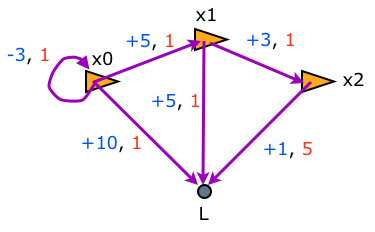
The ordered and measured distances are in blue; the weights of the equations are in red.
The constrains shown on the graph are:
- Initial position: \(x_0 = -3\)
- Relative measurement: \(L = x_0 + 10\)
- Relative pose: \(x_1 = x_0 + 5\)
- Relative measurement: \(L = x_1 + 5\)
- Relative pose: \(x_2 = x_1 + 3\)
- Relative measurement: \(L = x_2 + 1\). Weight = \(5\)
The weight of the equation of each of these constraints is 1, except the weight of the last measurement, which has a weight of 5, indicating that it is a particularly good measurement, i.e., it has a low variance of \(1/W = 0.2\).
Let’s dissect the scenario. The robot moves twice, taking a measurement from each location:
- It starts at x = -3, from which it observes the landmark at a distance of +10. This means that the landmark is close to -3+10 = 7.
- Then the robot moves +5 from which it observes the landmark at +5. This means that the robot should be close to -3+5 = +2 and the landmark should be close to 2+5=7, which matches the observation from the first location.
- Finally, the robot moves +3 from which it observes the landmark at +1. This means that the robot is at location 2+3 = 5 and the landmark should be close to 5+1=6, which does not match the observations from the first two locations.
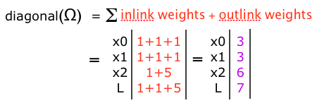
The \(\Omega\) matrix
To build the \(\Omega\) matrix, we could start by finding its diagonal. Each element of the diagonal is the sum of the weights of the incoming and outgoing edges to the particular node:
Then we can find the off-diagonal elements: for each edge i, j is the negative of the weight between node i and node j:
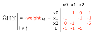
Thus we have the \(\Omega\) matrix:
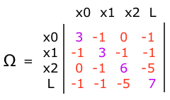
Also, an easy way to verify that the \(\Omega\) matrix is correct without drawing the graph is to add all the elements of a row or column. In the case of the initial position, the sum should add up to the weight of the initial position constraint. In the example, when adding the elements of the \(x_0\) row in \(\Omega\) we get
$$3 – 1 + 0 – 1 = 1$$
For every other constraint, either relative pose or landmark, the sum should be 0. In the example, when adding the elements of the row of \(x_2\) in \(\Omega\) we get
$$0 – 1 + 6 – 5 = 0$$
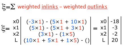
The \(\xi\) vector
The value of each element of \(\xi\) that corresponds to a node is the sum of the weighted incoming edges to the node minus the sum of the weighted outgoing edges:
Comment on the solution
This example was given in class but, although the derivation of the equations is correct, the setup of the equations has an error. Let’s see:
Solving \(\xi = \Omega X\) gives us
$$
\begin{eqnarray}
X &=& [x_0, x_1, x_2, L]^T\\
&=&[-3.000, 2.179, 5.714, 6.821]^T
\end{eqnarray}
$$
i.e., we estimated the landmark at 6.821 instead of 7, like the first two observations indicated. Also, we asked the robot to move +5 and +3 to 2 and 5 but apparently it made significant errors, and ended up at 2.179 and 5.714.
These results are a consequence of assigning a large weight to the last measurement; we assigned it a weight of w = 5, which sets the variance of the measurement to \(1/w = 0.2\), stating that the measurement was very good when, in reality, it was a very bad one.
If the last observation had been weighted as bad instead of good, i.e., if it had had a variance of 5 and a weight of \(w = 1/\mbox{variance} = 0.2\), then the results would have been
$$
\begin{eqnarray}
X &=& [-3.000, 2.050, 5.200, 6.950]^T
\end{eqnarray}
$$
Now everything fits: the bad measurement contributes less toward the solution than the good measurements so the estimates reflect what actually happened: the robot moved as commanded, with smaller errors than those estimated before, and now all the observations are consistent.
We can take the case to the extreme and assign to the last measurement a weight of 0.0001, indicating the measurement was lousy and its equation should be given almost no value when solving the system; then we would have gotten:
$$
\begin{eqnarray}
X &=& [-3.000, 2.000, 5.000, 7.000]^T
\end{eqnarray}
$$
i.e., the expected result for an essentially error-free scenario.
Code
The following code runs the three scenarios described above:
import numpy as np

np.set_printoptions(precision=3, floatmode='fixed')

def get_omega(w):
    # get the diagonal
    diag_0 = 3.
    diag_1 = 3.
    diag_2 = 1 + w
    diag_3 = 2 + w

    # now assemble the matrix
    omega = np.array([[diag_0,  -1., 0., -1.],
                      [-1., diag_1, -1., -1.],
                      [ 0., -1., diag_2, -w],
                      [-1., -1., -w, diag_3]])
    return omega


def get_xi(w):
    # get each term
    xi_0 = (-3. * 1) - (5. * 1 + 10. * 1)
    xi_1 = (5. * 1) - (5. * 1 + 3. * 1)
    xi_2 = (3. * 1) - (1. * w)
    xi_3 = (10. * 1 + 5. * 1 + 1 * w) - (0)

    # now assemble the vector
    xi = np.array([xi_0, xi_1, xi_2, xi_3])
    return xi


def solve_system(w_3):
    # our only param is w_3, which is the weight from x2 to the landmark
    omega = get_omega(w_3)
    xi = get_xi(w_3)
    X = np.linalg.solve(omega,xi)

    print("weight: ", w_3)
    print("omega:")
    print(omega)
    print("xi:", xi)
    print()
    print("X:", X)
    print("-----------------------------")


# set the weight of the last observation wrong, as if it had been good
w_3 = 5
X = solve_system(w_3)

# set the weight of the last observation correctly, as if it had been bad
w_3 = 1/5.  # w = 0.2
X = solve_system(w_3)

# set the weight of the last observation correctly, as if it had been lousy
w_3 = 0.0001
X = solve_system(w_3)
and yields the expected results:
~/Desktop:python ./graph-slam.py
weight:  5
omega:
[[ 3.000 -1.000  0.000 -1.000]
 [-1.000  3.000 -1.000 -1.000]
 [ 0.000 -1.000  6.000 -5.000]
 [-1.000 -1.000 -5.000  7.000]]
xi: [-18.000  -3.000  -2.000  20.000]

X: [-3.000  2.179  5.714  6.821]
-----------------------------
weight:  0.2
omega:
[[ 3.000 -1.000  0.000 -1.000]
 [-1.000  3.000 -1.000 -1.000]
 [ 0.000 -1.000  1.200 -0.200]
 [-1.000 -1.000 -0.200  2.200]]
xi: [-18.000  -3.000   2.800  15.200]

X: [-3.000  2.050  5.200  6.950]
-----------------------------
weight:  0.0001
omega:
[[ 3.000e+00 -1.000e+00  0.000e+00 -1.000e+00]
 [-1.000e+00  3.000e+00 -1.000e+00 -1.000e+00]
 [ 0.000e+00 -1.000e+00  1.000e+00 -1.000e-04]
 [-1.000e+00 -1.000e+00 -1.000e-04  2.000e+00]]
xi: [-18.000  -3.000   3.000  15.000]

X: [-3.000  2.000  5.000  7.000]
-----------------------------
~/Desktop: